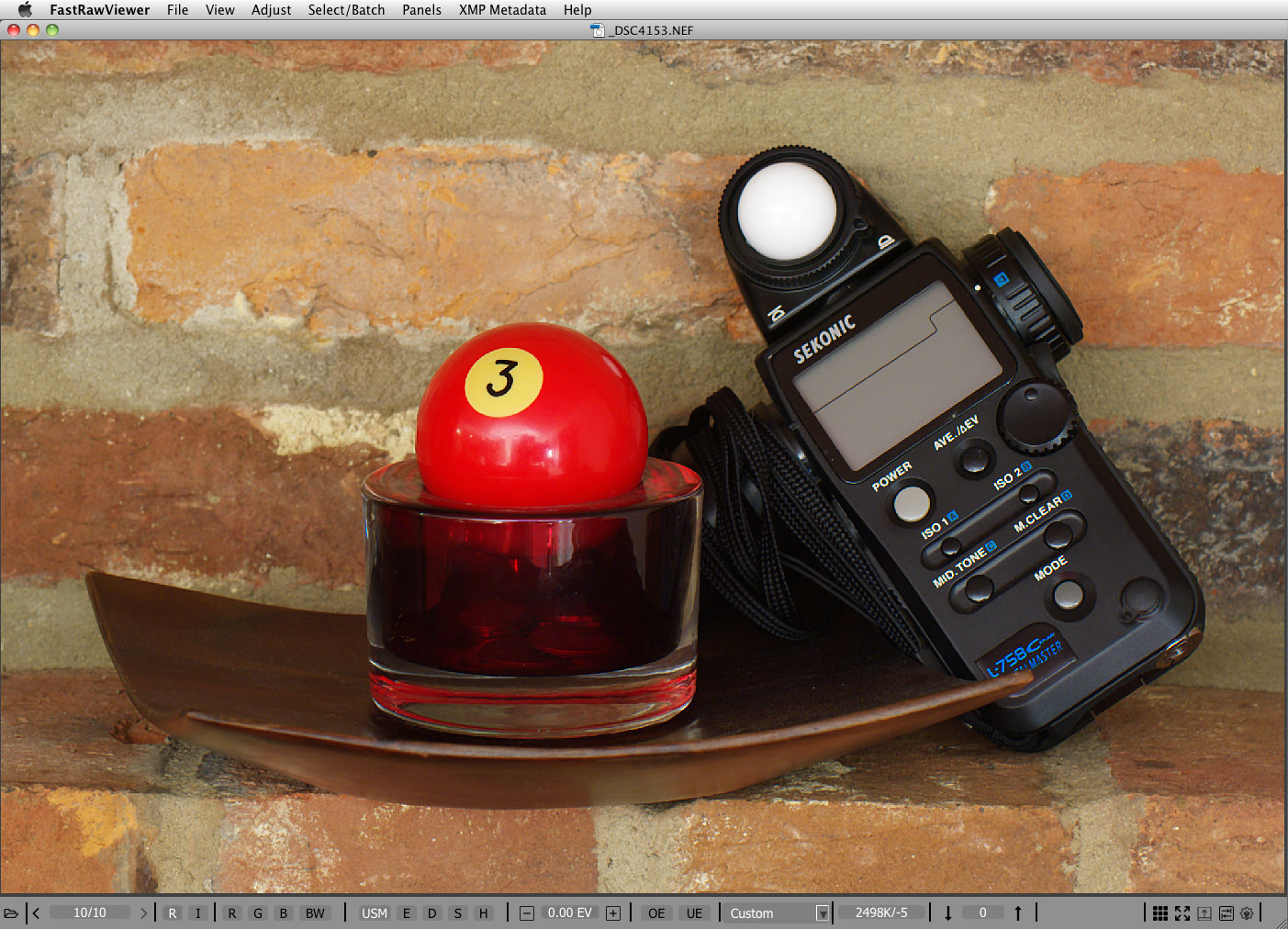
Suppose you have read somewhere that the dynamic range of your camera at a certain ISO setting is 11 stops. And here comes the immediate question – how can one use such a treasure to its full potential? Optimal exposure for RAW is the answer. But now we need to explain what we mean when we say, “optimal exposure for RAW”. Let’s start with one of the problems, which arises as a result of non-optimal exposure for RAW. Here is a typical wide dynamic range low-light scene. According to Sekonic spot-meter, it is wider than 11 stops:

Figure 1. FastRawViewer. Shot exposed 1 2/3 EV hotter than the in-camera exposure meter suggested.
We made two shots of the same scene – one (#4152) was exposed according to the in-camera exposure meter set to matrix metering mode. The other shot (#4153, Figure 1.) was exposed 1 2/3 EV hotter (spot-metered from white dome, for the procedure to determine the amount of correction please read on, or you can simply bracket). Matrix metering seems to have gotten fooled by the specular highlights on that white dome, hence it underexposed a little more than usual.
We opened them both in FastRawViewer, applied Shadow Boost to both of them to open the shadows, and applied +1.67 EV exposure correction to shot #4152 (the one that was exposed according to in-camera exposure meter recommendation, so that both of the shots had the same overall brightness).
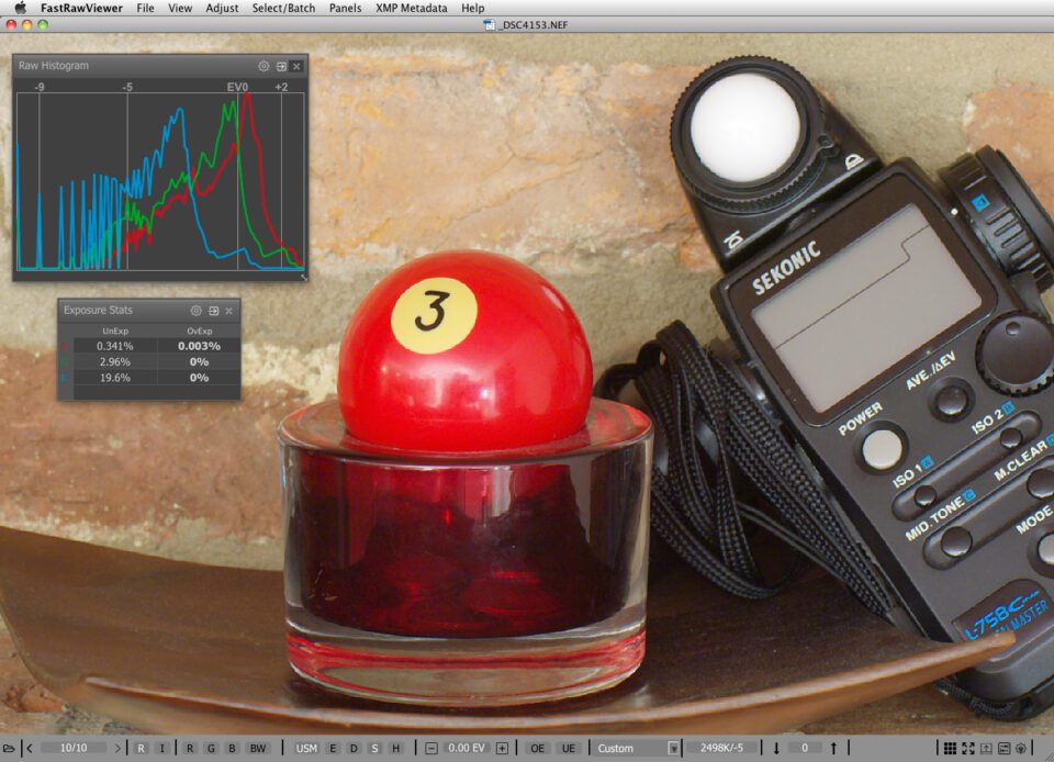
Figure 2. FastRawViewer. Zoom into shot #4153 with optimal exposure for RAW. Applied Shadow Boost.
As we can see on to the RAW histogram for shot #4153 (Figure 2) the capture definitely has more than 11 stops. Now we look at shot #4152.
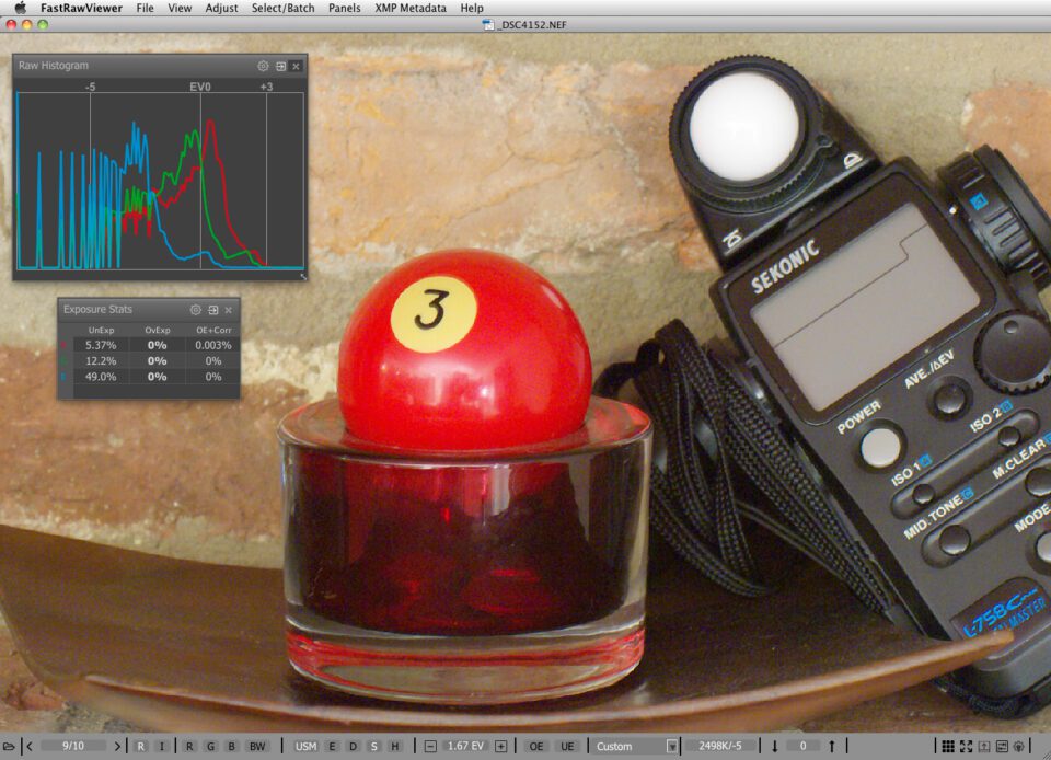
Figure 3. FastRawViewer. Zoom into shot #4152 that was exposed according to the in-camera exposure meter. Applied Shadow Boost and +1.67 EV exposure correction.
As we can see, shot #4152 exhibits significant noise everywhere below midtone. The thing with a camera’s dynamic range is that those exciting numbers become valid only when the signal reaches the maximum; that is, the exposure is the hottest possible for the given camera at a given ISO. Imagine a bucket having a volume of 2 gallons. If you do not fill it up to the top, some volume is wasted. It’s the same with a camera. If your whitest white is not exposed to the maximum, the top portion of the dynamic range is not being used. This immediately means that in order to use the dynamic range of the camera to its fullest and simultaneously to have as little shadow noise as possible, the whitest whites where you want to keep some texture details need to be exposed so that they are just below clipping. In a sense, one can say that dynamic range characterizes the depth, and starts from the top, while the bottom is sort of fuzzy because of individual tolerance to noise, viewing conditions, size of the output, etc.
Back to our bucket analogy – if one tries to pour, say, 2.5 gallons in it, an overflow happens, and half a gallon will end up on the floor. In digital photography we know this as highlight clipping. That is, if we try to expose a pixel hotter than its capacity allows, everything that is above the capacity will pour out, causing blown-out highlights. By the way, if one tries to set exposure low to keep from clipping all the light sources and specular highlights, he is, most probably, also wasting a couple of stops of dynamic range.
Unfortunately the metering systems of our cameras are not designed to provide the proper placement of the highlights right out of the box (this is partially because to do so, the camera’s AI needs to make a guess as to what a photographer considers to be “important highlights”, and if it guesses wrongly, it may arrive at an unacceptable exposure). One can try different metering modes with the camera, with mixed results when it comes to optimal exposure for RAW. You can use RawDigger or FastRawViewer to see how close you are; be prepared for more misses than hits, in part because the complex metering modes are optimized for JPEGs rather than for RAW. Reliability and repeatability, however, come with manual metering in the spot meter mode. While placing important highlights at the top, let’s take advantage of one very well-known and stable feature of the camera: cameras are calibrated in such a way as to provide the exposure that will result in the rendering of whatever was under the spot meter as “middle grey”.
For a JPEG middle grey is defined as 118 RGB in sRGB color space, which corresponds to the proverbial 18% grey (and L* = 50 in Lab color model, too). For RAW, middle grey is not fixed by common standards, and camera makers have some freedom while placing it. Why is this so? Modern cameras have relatively low noise, and customers often complain that the highlights in their exposures are blown out. To provide extra room for the highlights, camera makers tend to calibrate the exposure so that it shifts middle grey down to 13% (instead of 18%), and often even lower than that. This is what often causes the rumors that camera makers cheat with ISO. In fact it is not cheating, because in most cases the ISO speed is defined for the processed output (JPEG) and not for RAW. Lets look at the shots of the scene we have already used in the article “Why Bother Shooting RAW if Culling JPEGs?”.

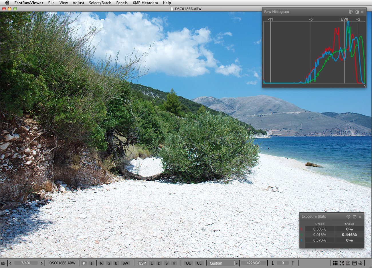
Figure 4. FastRawViewer. Scene with a high dynamic range. Shot #1866 with optimal exposure for RAW (ETTR).
Shot #1861 was exposed according to the in-camera exposure meter and it has the hottest possible exposure for JPEG. Shot #1866 had exposure increased by 1 2/3 EV, and it has the optimal exposure for RAW (ETTR). If we look at the shadows of those two shots after running them through ACR (shot #1866 was converted without any adjustments; while shot #1861 was converted with +1.67 exposure correction applied in ACR, to “match” the exposure difference between the shots), we see that there’s quite a difference in the shadows between these two shots. By the way, the smaller the sensor is, the more difference optimal exposure will make.
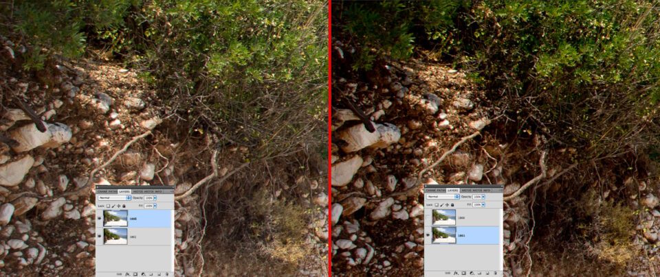
Figure 5. Photoshop. Left part – shadows in shot #1866 after conversion in ACR. Right part – shadows in shot #1861 after conversion in ACR with +1.67 EV exposure correction
A tone curve applied when rendering a JPEG takes care of matching of whatever the middle grey is in RAW to the standard 18% grey in JPEG. But if we are shooting RAW and trying to exploit the dynamic range of our cameras to its full potential we need to set an exposure which is close to optimal, and place the highlights in the RAW where they belong – at the top of the dynamic range of your camera.
In other words, the top of the dynamic range of the scene (and by scene we mean everything you want to capture, and not the irrelevant / specular highlights) needs to be placed at the top of the dynamic range of the camera.
Back to the question of achieving this goal in a reliable and repeatable manner:
- First, we need to know the value for the middle grey in RAW numbers. This varies by camera model and sometimes by ISO setting.
- Next we need to know the maximum value that the RAW file may contain. This also varies by camera model and may depend on ISO setting; it may be the same as the maximum value for ADC (12 bits, 4095; 14 bits, 16383), or it may be less.
- Finally we need to calculate the result – the number of stops between the middle grey in RAW and the maximum in RAW for this specific camera and given ISO setting, to use this number as the exposure compensation when metering off the highlights that we want to keep.
Again, to use the result we need to meter from the whitest white in the scene where we want to preserve some texture and details, and apply exposure compensation in the camera that equals the number we have just determined. Consequently, the important whitest whites of the scene will receive the maximum allowed exposure, thus being placed at the top of the dynamic rage of the camera. This way you have achieved optimal exposure, also known as ETTR. The whole thing hinges on the theory that whatever is presented to an exposure meter will be recorded as middle grey as soon as the exposure meter recommendations are followed. Let’s check this theory.
We made six shots of the ColorChecker (Figure 1):
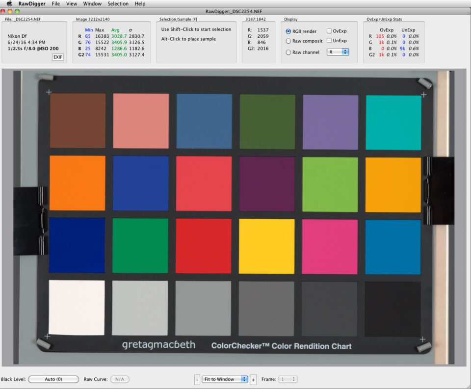
Figure 6. RawDigger. ColorChecker CC24
For each shot, we spot-metered one of those neutral grey patches at the bottom row, starting from the white patch, setting the exposure according to the recommendations of the spot meter. Next, we opened those shots one by one in RawDigger, sampled the patch we spot-metered, and checked the RAW values for this sample.
As you can see, the RAW values for the patch under the meter are very close to each other:
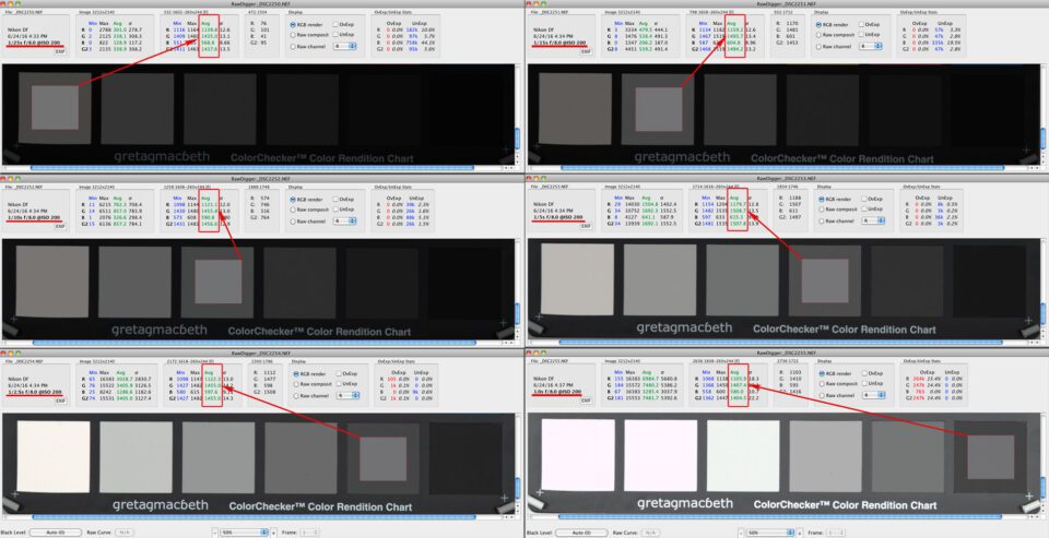
Figure 7 – RawDigger. RAW values for the 6 shots exposed as per spot meter readings from respective patches
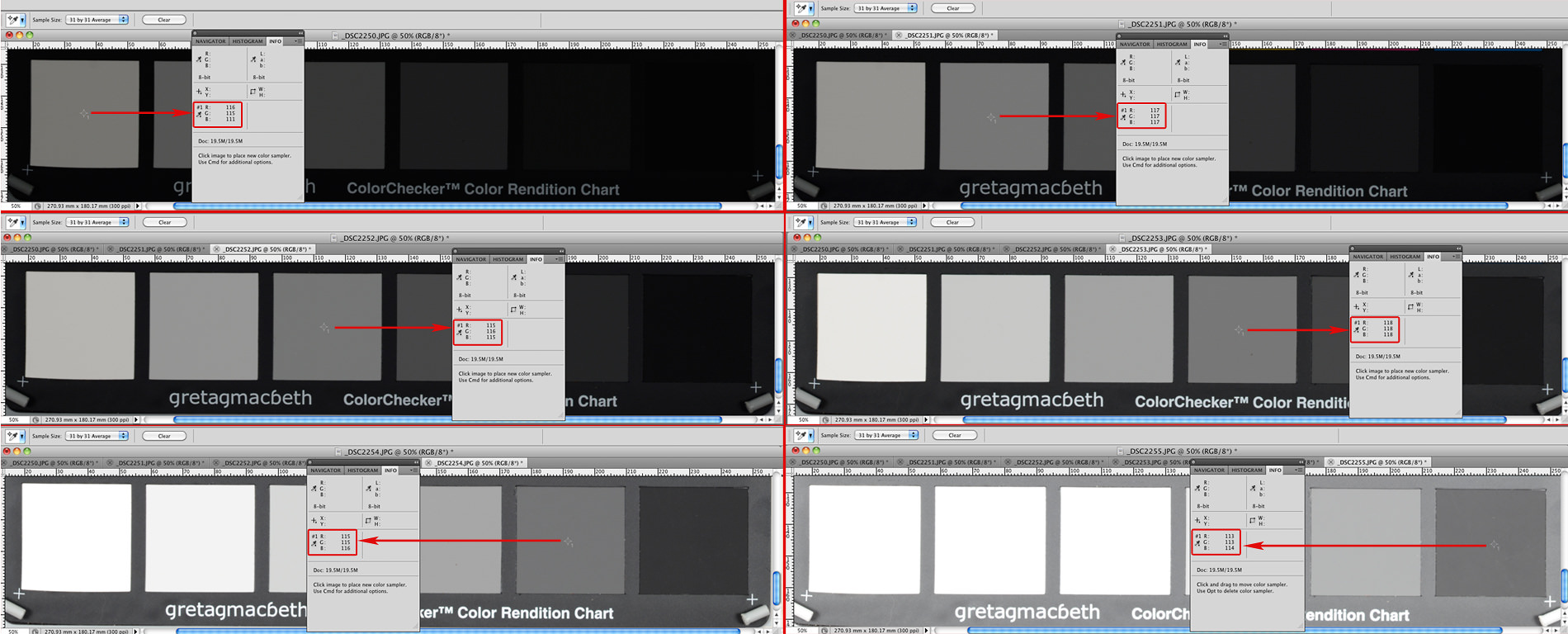
Because the camera was set to record both RAW and JPEG, we can check the RGB values in Photoshop too. As expected, they also turned to be very close to each other and to the target value for the mid-tone for JPEG, RGB=118.
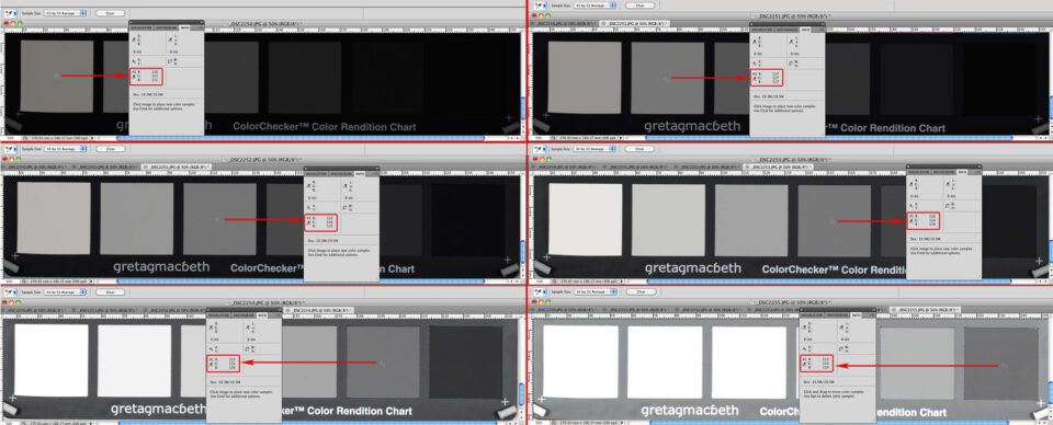
Figure 8 – Photoshop. RGB values from OOC JPEGs of the same 6 shots.
Now that we are confident that the spot meter indeed guides the exposure in such a way that whatever shade of grey we put under the spot meter, the result will be the same number in RAW, with the number representing middle grey in terms of camera calibration for RAW. Because the theory proves to be true, you don’t need to meter and shoot all 6 patches: one is enough, or you can use a grey card.
- To get the most accurate reading for the middle grey in RAW, it is more practical to use a light grey patch / card (ColorChecker Passport has a separate grey page for white balance, it has L*=81, or, in other words, it is 60% grey, light enough to use with confidence) or matte white. The reason for using lighter tones is to keep flare as low as possible for both metering and capture. The higher reflection values of the lighter samples are less prone to flare compared to lower reflection values for dark grey and black samples.So to get GMiddleGrey, make a shot with exposure setting according to the spot meter recommendation for a white or a light grey patch, open the shot in RawDigger, place a sample on the patch from which you metered, and read average value for the Green channel, Avg G. In our case, GMiddleGrey = 1435.
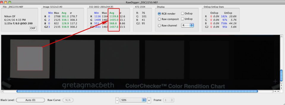
Figure 9 – RawDigger. Reading middle grey value for RAW
- Now let’s determine the maximum value for the G channel that RAW can contain (maximum values may be different for different channels).
There are basically 2 ways to determine the maximum:
- One way, which does not require additional shots, is to include from the beginning some source of relatively small specular highlights in the scene (a shiny metal ball, for example, is what is often used); however, this can create flare in the shot, and that flare will throw the metering off; maybe just a little, but sometimes significantly.
- The other way is to simply shoot with long exposure, ensuring that part of the shot reaches clipping.
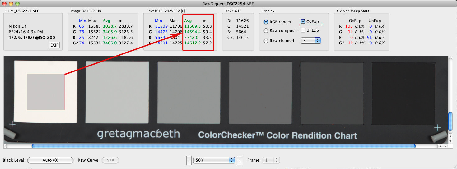
The truly clipped region will usually have a very small sigma (σ, standard deviation, Std.Dev.) value, in the order of single digits, in many cases very close to 0. The mean (average, Avg) value of the green channel for the clipped region is the maximum raw value we are after. On Figure 5, the average for green (Avg G) is 14,594.4; the standard deviation for green (σG) is 59.4. This means that there is no clipping.
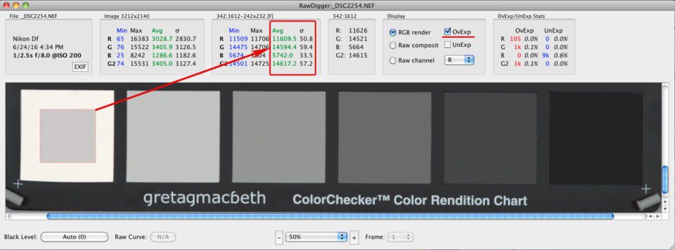
Figure 10 – RawDigger. Shot #2254. Large sigma (σ) values for all channels
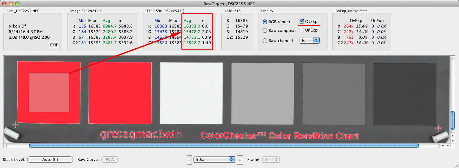
On Figure 6, the average for green (Avg G) is 15,478.7; the standard deviation for green (σG) is 2.03. That is the G channel clipping all right, and increasing exposure further will not help decrease σG in any significant manner – see the next Figure, #7.
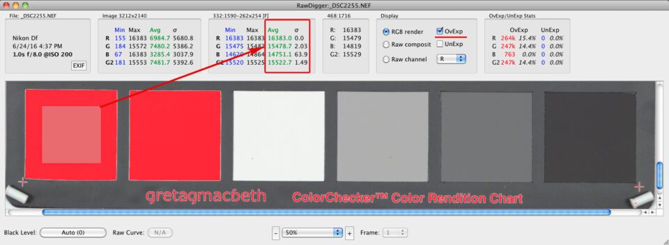
Figure 11 – RawDigger. Shot #2255. Small sigma (σ) value in Green (and Red) channels
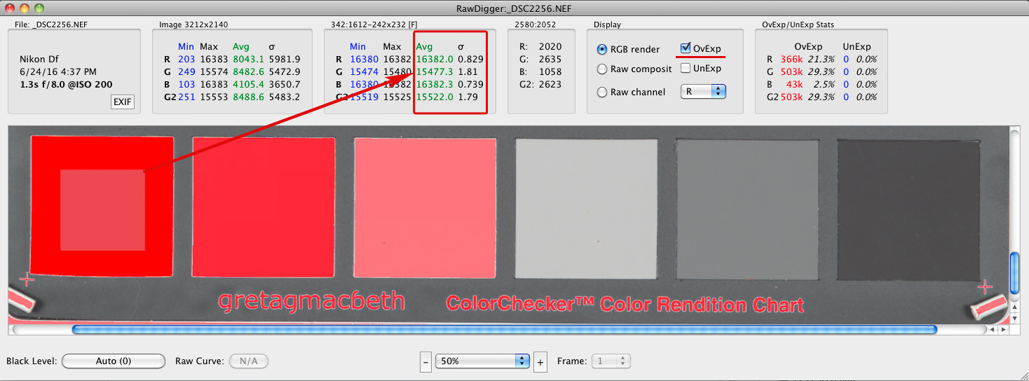
On Figure 7, the average for green (Avg G) is 15,477.3; the standard deviation for green (σG) is 1.81; that is, the green channel G is clipped, like it is on the previous one:

Figure 12 – RawDigger. Shot #2256. Small sigma (σ) values in all channels
Nevertheless, the Avg G from the previous shot, #2255 (Figure 6) is a better choice: as you can see the Avg G is larger here, and this is because we triggered intense anti-blooming on shot #2256 (Figure 7), and it acts like solarisation, also known as a Sabattier effect. On film, increasing exposure results in decreased density of the negative; however, it is much milder on digital.
So, we will consider Avg G for a sample area from shot #2255 (Figure 6) as maximum raw value: Gmax = 15,478.7
- Finally, let’s calculate the value of exposure compensation (the number of stops, EV, between the middle grey in RAW and maximum / clipping point in RAW) for the given camera at a given ISO. We are going to use the formula:
EV = log2(GMax / GMiddleGrey) (1)If you are interested in what the corresponding percent of grey is, you can calculate it as
percent = 100% * GMiddleGrey / GMax (2)In our case GMiddleGrey = 1435 and Gmax = 15,478.7, so using the formula (1a) we get
log2(15,478.7 / 1435) ≈ 3 1/3 EVThat is this value of exposure compensation turns to be +3 1/3 EV (meaning the calibration for our camera puts the mid-tone in raw to 9.27%, nearly a stop lower than the “expected” 18%).Let’s shoot with calculated exposure compensation and see… For the next shot #2257, we metered off the white patch, applying to the meter readings the exposure compensation we just determined, +3 1/3 EV. Now we open it in RawDigger and check raw values of the white patch:
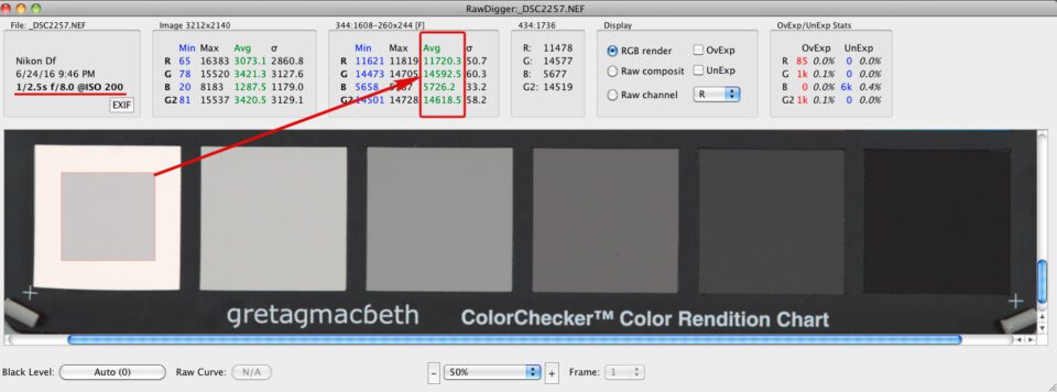
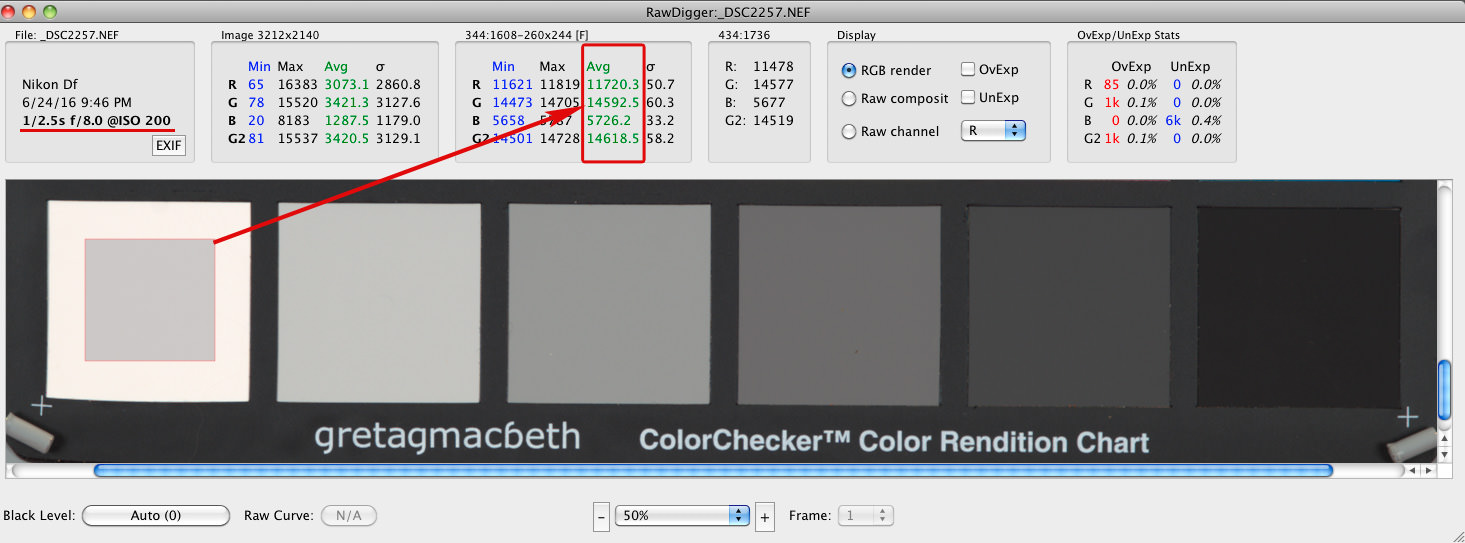
Figure 13 – RawDigger. Shot #2257 made with calculated exposure compensation +3 1/3 EV. RAW
As you can see, for a white patch average RAW value for Green channel (Gavg) is 14592.5. That is we are very close to the clipping point but still below it.
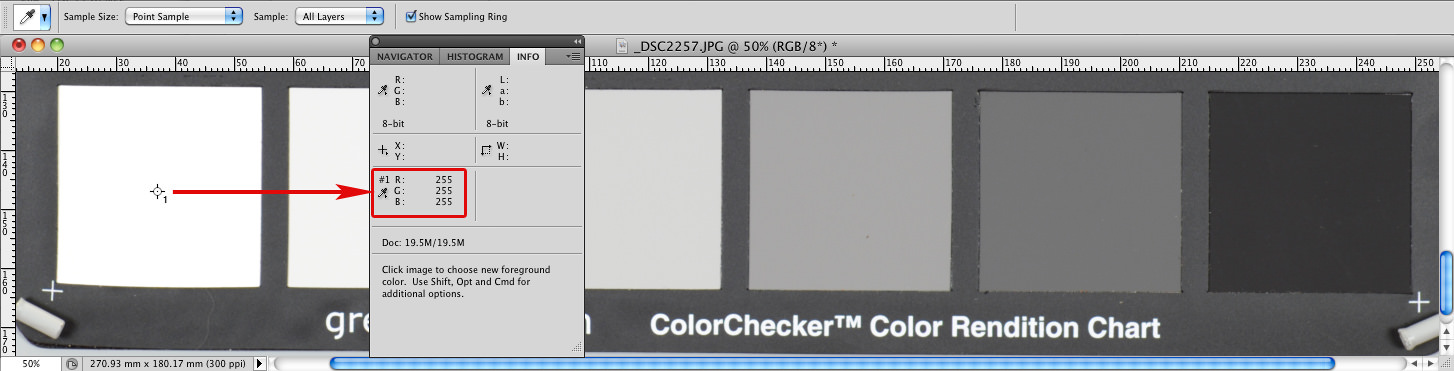
If we look at the JPEG of the shot #2257 (Figure 9) we will see that we “overexposed”: R=G=B=255. That is, of course, not so. OOC JPEGs do not use the full dynamic range available in RAW.
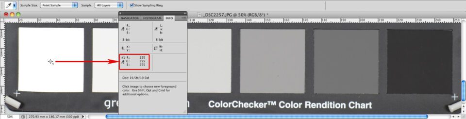
Figure 14 – Photoshop. Shot #2257 made with calculated exposure compensation +3 1/3 EV. OOC JPEG
If you hate calculations, you can use a brute force approach. Shoot some neutral patch or grey card, setting the exposure as per your camera’s spot-meter recommendations and start adding exposure compensation, EC (you can set EC initially to +2 1/3 EV, which corresponds to calibration of the mid-tone in raw to 20% grey; we suggest this because calibration shouldn’t be higher than 20%) until the raw values for the patch or card comes close to clipping, within 1/3 EV from it. Incidentally, you can often hear advice to meter off of the 18% grey card to set the correct exposure. This exposure is not likely to be optimal for raw, as in most cases it does not place the highlights high enough on the DR scale.
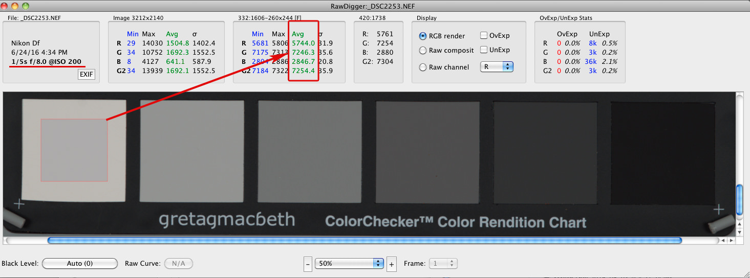
Shot #2253 was metered from the N5 patch of ColorChecker with zero exposure compensation, which by design has L*=50, or, in other words, it is 18% grey. As you can see in RawDigger, the white patch is recorded 1 stop below clipping, and we have not achieved optimal exposure (Figure 10). Not even close.
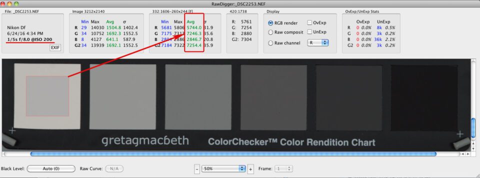
Figure 15 – RawDigger. Shot #2253. RAW. Metered from N5. White is one stop below maximum
If we check OOC JPEG for the same shot (Figure 11) we will see that while middle grey was correctly placed at 118 (sample 2), the RGB values for the white patch (sample 1) are (220, 220, 225), that is, seriously below maximum value.
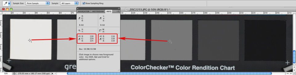
Figure 16 – Photoshop. Shot #2253. OOC JPEG. Metered from N5. White is below maximum
Sekonic 758 in incident metering mode recommended 1/4s for shutter speed, matrix and center-weighted metering in the camera suggested 1/6s and 1/5s, respectively, while the shutter speed for ETTR, as we already know from shot #2257, is 1/2.5s. All out-of-the-box metering turned to be inefficient in terms of ETTR, but very consistent with the ≈1 EV difference we observed between calibration for raw for this camera (≈9%) and calibration for JPEG (≈18%).
We are very happy to hear that a new camera has ½ of a stop more DR than a previous model. We consider those ½ stop to be a huge improvement. However, if we are not using ETTR, we will be getting from this new camera the same or even lower image quality an ETTR practitioner is getting from the previous model.
The post How to Use the Full Dynamic Range of Your Camera appeared first on Photography Life.
Photography Life